Event-based Visual Odometry and Inertial Odometry
1. Event-based Visual Odometry (VO)
Event-based Visual Odometry (Event VO) is a paradigm that leverages asynchronous event cameras to estimate motion. Unlike traditional frame-based cameras, event cameras output brightness changes at pixel-level with microsecond resolution.
Key Features
- High temporal resolution (microseconds)
- Low latency and no motion blur
- High dynamic range
Event Generation Model
Event cameras respond to changes in logarithmic brightness rather than absolute intensity. An event is triggered when the change in log intensity exceeds a predefined threshold.
$$ \frac{d}{dt} \left( \log I(u,v,t) \right) \geq C $$where \(I(u,v,t)\) is the image intensity at pixel \((u,v)\) and time \(t\), and \(C\) is the contrast threshold.
The polarity of the event is defined as:
$$ p = \begin{cases} +1 & \text{if } \frac{d}{dt} (\log I) \geq C \\ -1 & \text{if } \frac{d}{dt} (\log I) \leq -C \end{cases} $$Thus, each event is represented as \(e = (u, v, t, p)\). This representation makes event cameras invariant to absolute illumination and highly responsive to motion.
Sensor Used: Event VO commonly uses Dynamic Vision Sensors (DVS) or DAVIS cameras.
Limitations
- Requires motion to generate events
- Sparse data in static environments
- Challenging outdoors due to noise and illumination variation
- Works better indoors due to controlled lighting
2. Neuromorphic Sensor: DAVIS 240C
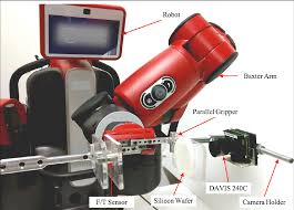
The DAVIS 240C sensor combines a standard frame-based camera with an event-based sensor.
Key Characteristics
- Resolution: \(240 \times 180\)
- Outputs both frames and events
- High temporal resolution (events)
- APS grayscale frames available
3. UZH DAVIS 240C Dataset
The DAVIS 240C dataset from UZH provides synchronized multi-modal data for visual-inertial odometry.
Available Data
- RGB Images – Frame-based grayscale images
- events.txt – Asynchronous event stream \((u,v,t,p)\)
- groundtruth.txt – 6-DoF poses
- camera_calib.txt – Intrinsic calibration parameters
- imu.txt – IMU measurements (accelerometer + gyroscope)
The ground truth is represented as: \(\text{Pose} = (t_x, t_y, t_z, q_x, q_y, q_z, q_w)\). This dataset enables both Event VO and Event-based Visual-Inertial Odometry (VIO).
4. Experiment 1: Understanding Event Sensor Readings
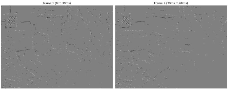
Events are accumulated over fixed time windows (30ms) to generate event frames.
Pipeline
- Read events from 0–30ms (Frame 1)
- Read events from 30–60ms (Frame 2)
- Create image grid of size \(H' \times W'\)
- Accumulate events based on polarity
5. Experiment 2: Event-driven VO
Pipeline
- Read events.txt
- Generate time surfaces (Frame 1 and Frame 2)
- Track features using SSD patches
- Normalize using camera intrinsics
- Estimate Essential matrix using 8-point method
- Recover pose
- Compare with ground truth (RRE, RTE)
| Pair | Features Tracked | Min RRE (°) | Min RTE (°) |
|---|---|---|---|
| 0 → 1 | 42 | 3.6075 | 70.2578 |
| 1 → 2 | 22 | 1.1908 | 75.7862 |
| 2 → 3 | 35 | 14.8443 | 88.1986 |
| 3 → 4 | 93 | 1.9156 | 10.1369 |
| 4 → 5 | 87 | 0.5051 | 61.3960 |
| Mean | -- | 4.4127 | 61.1551 |
Observations
- Low Relative Rotation Error (RRE)
- High Relative Translation Error (RTE)
- Reason: Limited epipolar-consistent matches
6. Experiment 3: Event VO with Increased Temporal Window (100ms)
In this experiment, the temporal window for event accumulation is increased from 30ms to 100ms to improve feature correspondences.
Pipeline
- Read events from
events.txt - Accumulate events in two windows: Frame 1: \(t \in [0, 100]\) ms and Frame 2: \(t \in [100, 200]\) ms
- Generate time surfaces for both frames
- Detect features on Frame 1 (e.g., corners or high gradient regions)
- Track features to Frame 2 using SSD-based patch matching
- Normalize matched keypoints using camera intrinsics: \(x_n = K^{-1} x\)
- Estimate Essential Matrix using 8-point algorithm
- Recover pose \((R, t)\) from Essential matrix
- Compare with ground truth to compute RRE and RTE
Key Insight
Increasing the temporal window results in: Higher event density, more feature correspondences, and improved epipolar consistency.
| Pair | Features Tracked | Min RRE (°) | Min RTE (°) |
|---|---|---|---|
| 0 → 1 | 64 | 2.8065 | 68.8572 |
| 1 → 2 | 42 | 0.9701 | 71.2876 |
| 2 → 3 | 55 | 10.5619 | 84.6981 |
| 3 → 4 | 106 | 1.1219 | 8.9631 |
| 4 → 5 | 98 | 0.38412 | 63.0639 |
| Mean | -- | 3.0917 | 59.3739 |
Observations
- Significant reduction in RTE
- Slight improvement in RRE
- Better stability in pose estimation
Limitation
- Larger time windows introduce motion blur in event aggregation
- Trade-off between temporal resolution and feature richness
7. Experiment 4: Robust Estimation using RANSAC and MAGSAC++
This experiment introduces robust estimation techniques to handle outliers in feature correspondences.
Pipeline
- Generate time surface images (same as Experiment 3)
- Detect and match features using SSD-based patch matching
- Normalize matched keypoints using camera intrinsics
- Apply robust estimation: RANSAC with \(k = 100\) iterations and MAGSAC++ with adaptive thresholding
- Estimate Essential Matrix for inlier correspondences
- Recover relative pose \((R, t)\)
- Compute RRE and RTE using ground truth
| Pair | Total Features | RANSAC (RRE / RTE) | MAGSAC++ (RRE / RTE) |
|---|---|---|---|
| 0 → 1 | 42 | 1.88° / 83.27° | 1.92° / 80.19° |
| 1 → 2 | 22 | 3.44° / 77.41° | 2.82° / 89.97° |
| 2 → 3 | 35 | 1.03° / 64.44° | 2.85° / 75.86° |
| 3 → 4 | 93 | 4.13° / 14.60° | 2.42° / 18.97° |
| 4 → 5 | 87 | 0.43° / 63.82° | 1.17° / 81.56° |
Observations
- RRE remains low for both methods
- RANSAC provides more stable translation estimates
- MAGSAC++ shows higher RTE due to sensitivity to sparse event matches
8. Experiment 5: Hough Transform-based Corner Detection
This experiment replaces standard feature detection with Hough-based corner detection tailored for event frames.
Pipeline
- Generate time surface images (100ms window)
- Apply Hough Transform to detect corner-like structures
- Extract keypoints from Hough space
- Track features between frames using SSD patches
- Normalize matched keypoints
- Estimate Essential Matrix (8-point method)
- Recover pose \((R, t)\)
- Compute RRE and RTE
| Pair | Hough Corners Matched | RRE (°) | RTE (°) |
|---|---|---|---|
| 0 → 1 | 17 | 171.11 | 71.24 |
| 1 → 2 | 17 | 45.60 | 71.28 |
| 2 → 3 | 38 | 4.35 | 61.20 |
| 3 → 4 | 30 | 4.54 | 16.32 |
| 4 → 5 | 26 | 32.39 | 67.36 |
Observations
- Inconsistent feature detection across frames
- Poor repeatability of Hough corners
- Unstable RRE and RTE
9. Experiment 6: Direct Event-based Visual Odometry
Instead of relying on discrete features, this method directly uses intensity variations from event frames.
Pipeline
- Generate time surfaces for consecutive windows
- Initialize pose estimate \((R, t)\)
- Define photometric error between warped event frames
- Optimize pose by minimizing: \(\sum || I_1(u,v) - I_2(\text{warp}(u,v, R, t)) ||^2\)
- Iterate optimization using gradient-based methods
- Output optimized pose
- Compute RRE and RTE
| Frame Pair | RRE (°) | RTE (°) |
|---|---|---|
| 0 → 1 | 33.26 | 87.10 |
| 1 → 2 | 4.37 | 78.14 |
| 2 → 3 | 113.81 | 46.45 |
| 3 → 4 | 33.42 | 88.32 |
| 4 → 5 | 6.50 | 125.43 |
| Metric | Value |
|---|---|
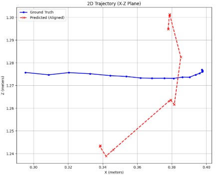
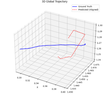
| ATE (RMSE) | 0.0328 m |
| APE Translation (Mean) | 0.0307 m |
| APE Rotation Vector (RMSE) | 145.9184° |
Observations
- More stable motion estimation compared to feature-based methods
- Sensitive to initialization and noise
10. Experiment 7: Direct Event-based Visual-Inertial Odometry
This experiment integrates IMU data with direct event VO for improved robustness.
Pipeline
- Read IMU data (angular velocity, acceleration)
- Integrate IMU to obtain motion prior
- Generate time surface images
- Use IMU prior to initialize pose
- Minimize photometric error with IMU regularization: \(E = E_{\text{photometric}} + \lambda E_{\text{IMU}}\)
- Optimize pose \((R, t)\)
- Compute RRE and RTE
Visualization Results
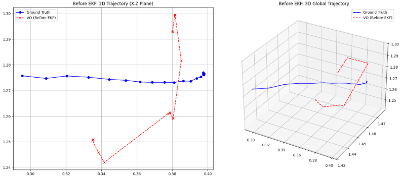
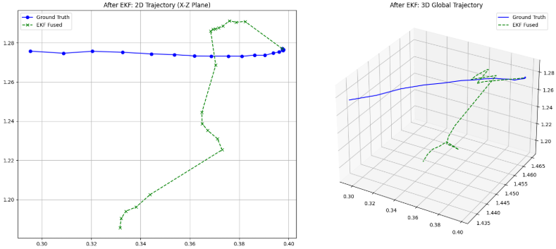
Observations
- Reduced drift compared to pure VO
- Improved stability in translation estimation
Conclusion
Event-based Visual Odometry demonstrates strong performance in high-speed and high dynamic range scenarios. While feature-based methods suffer from sparse correspondences, increasing temporal windows improves robustness. Direct methods and sensor fusion (VIO) further enhance accuracy. However, challenges remain in translation estimation due to limited epipolar constraints and noise sensitivity.