Visual SLAM Experimentation

Abstract

This webpage highlights experimentation in Visual SLAM using Graph-based Pose Regression Modules across two diverse datasets: the Tea Forest dataset and the KiTTi 2012 SLAM Benchmark (Seq 02). In this framework, the outputs of the Visual SLAM module rely entirely on the absolute pose—converted from the Regressed Pose—to perform 3D reconstruction. Depending on the dataset, the depth maps required for mapping are obtained either through Monocular Depth Estimation (MDE) or Stereo Disparity Matching.

Visual SLAM Pipeline

The Visual SLAM pipeline used in these experiments is designed to process video into 3D environments efficiently. The workflow is structured as follows:

1. Data Initialization: The system loads video frames (or an image sequence) along with the camera's intrinsic parameters and available depth data.
2. Stereo Initialization: A pair of consecutive images is passed into the algorithm to establish an initial relationship between frames.
3. Feature Detection & Matching: We utilize LoFTR, a dense, detector-free deep learning method, to reliably identify and match keypoints across the image pair.
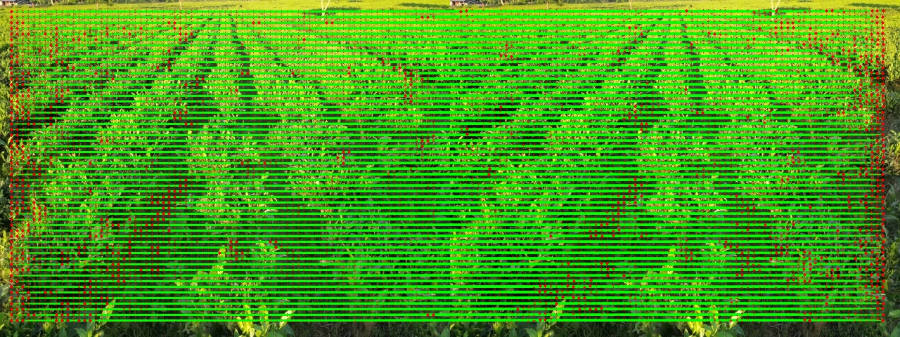
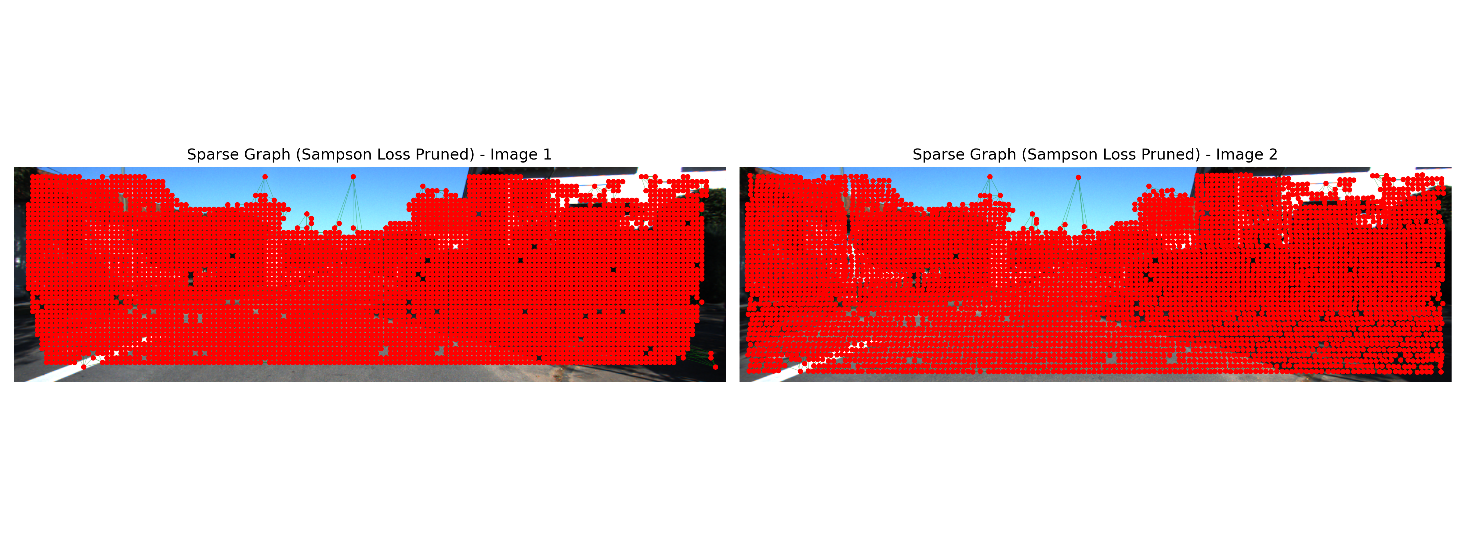
4. Graph Construction & Pruning: The raw matches are converted into a spatial graph using a K-Nearest Neighbors (K-NN) method. To remove incorrect matches (outliers), we filter the graph using geometric constraints—specifically an initial estimate of the essential matrix combined with a Sampson Distance threshold. This results in a clean Sparse Graph.
5. Relative Pose Estimation: The Sparse Graph is fed into a Graph Relative Pose Estimation module. This network outputs the predicted movement between the two frames as relative quaternions and translation vectors.
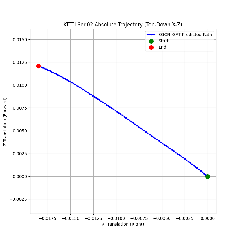
6. Absolute Pose Tracking: Assuming the autonomous system begins at a designated origin, we chain these consecutive relative poses together using transformation matrices. This accumulation yields the camera's Absolute Pose (its continuous trajectory in the world).
7. Mapping: Using the calculated Absolute Pose, image pixel coordinates, and depth maps (either calculated on-the-fly or loaded from memory), the system maps the environment in 3D space. (Note: Additional drift-reduction techniques like Pose Graph Optimization (PGO) and scale estimation exist but are not implemented in this specific iteration).
8. 3D Reconstruction: The final output is a dense 3D map, typically voxelized using OctoMap or passed down to a Gaussian Splatting module for rendering.

Tea Forest Dataset

For this experiment, the provided inputs were the raw video and camera intrinsics. Because this is monocular data, depth was calculated using a Monocular Depth Estimation approach (the Distill Any Depth module). A Graph-based pose estimation network alongside an absolute pose accumulator was deployed to calculate the trajectory.

Input Video

Feature Matches

Reconstruction with Trajectory

Loading 3D Model...

Interactive 3D Reconstruction

Download tea_octomap.ply

KiTTi 2012 SLAM Benchmark

This experiment utilized Sequence 05 of the KiTTi benchmark, processing video and camera intrinsics. Because KiTTi provides stereo vision data, depth was calculated accurately using stereo disparity matching. Graph-based pose estimation was performed using a hybrid GCN-GAT (Graph Convolutional Network - Graph Attention Network) module, followed by absolute pose calculation.

Input Video (kitti_video.mp4)

Feature Matches (LoFTR)

Estimated Trajectory (Absolute)

Graph Output (Sparse Graph)

Trajectory and 3D Reconstruction

Octomap (Cloud Compare)

Loading 3D Model...

Interactive 3D Reconstruction (Octomap)

Download kitti_octomap.ply

Conclusions

The outputs from these experiments clearly demonstrate improved 3D reconstruction when strict epipolar geometry is enforced within deep learning-based pose estimation models, leading to notably reduced drift. In the future, the tighter integration of depth maps and optical flow maps could further refine pose calculations, ultimately yielding higher-fidelity 3D environmental reconstructions.